Optimum Shading Device
A construction method using AutoCAD 2000
by Thanos N. Stasinopoulos
 
The design of a shading device is a rather complicated task with many parameters involved, from solar geometry to aesthetics or maintenance.
A major issue here is the balance between opposite seasonal requirements: A fixed device that protects a window during summer reduces solar gains & daylight during winter too.
A. & V. Olgyay in 'Solar Control & Shading Device' (Princeton University Press, 1957/1976) propose a design approach to optimize the performance of a shading device i.e. to maximize shading in summer and minimize it in winter: They use a matrix of hourly ambient temperatures above a set limit (e.g. 20oC) as a guide to the optimum shading mask.
Similarly, E. L. Harkness & M. L. Mehta in 'Solar Radiation Control in Buildings' (Applied Science, 1978) present a method to construct an 'optimum' shading device, which offers full protection during certain months and less during the rest: Using the lowest sun path of the warm season, they employ Descriptive Geometry techniques to remove the portion of a selected shading surface that blocks solar rays in winter only.
Of course solar protection is not just a matter of blocking the direct solar rays: Closely related issues like diffuse & reflected irradiance, infrared energy emitted by the shading device itself, air movement, or effects on daylight, glare & view, need to be addressed too.
Nevertheless, the geometric aspects of shading design are rather complicated, especially if one wishes to study alternatives or seasonal performance. A solid modeler like AutoCAD 2000 can make things much easier, as explained below.
The method shown here utilizes AutoCAD functions related to solar geometry and solid modelling for the construction of a shading device that fully shades a given opening during a selected period.
Following the Harkness & Mehta approach, the idea is to construct a set of prismatic volumes containing the solar rays that intercept the opening through the day. These volumes are used to determine the minimum portion of a shading solid that shades the opening during the chosen date and when the sun moves even higher.
The user should first select the 'summer threshold' date according to climatic conditions and building type & use. In this decision, the different annual symmetries of ambient temperatures & solar movements impose a compromise between the seasonal requirements for shading & solar access: In the north hemisphere, reduced solar access might be beneficial in warm September but not in cool March, although the sun paths are identical.
Depending upon the daily schedule of the building use, one could specify the required Daily Shading Period, say from 9 am to 5 pm.
There is no need for a complete 3D model of the building, just a 3D planar shape representing the opening is enough -unless the study will include adjacent building volumes.
The final output can be used as a guidance for the proper geometry of a fixed shading device that features an organic minimalism.
In the following description, the red words denote AutoCAD terms.
 
Phase 1 Prepare model
#1
Rotate your model so North coincides with the WCS angle origin (right-hand side of the screen). This is in order to avoid frequent changes of UCS in following steps.
#2
On the plane of the opening which is to be shaded, draw a Rectangle or other 2D Polyline along its perimeter. This is referred as Opening Contour below.
Phase 2 Find solar angles
#3
For each hour of the Daily Shading Period:
  • Use command Lights to create a New Distant Light.
  • Invoke the Sun Angle Calculator option and input the required data.
  • Note the solar Azimuth & Altitude angles as shown.
#4
Repeat the process of #3 for all hours of the Daily Shading Period and create a table of solar altitude & azimuth angles.
Sun Angle Calculator measures positive azimuth angles (w) in the opposite direction than the typical AutoCAD norm, therefore you should modify the w values: If w is positive then change to 360-w, else –w.


Excel table
 

Phase 3 Construct hourly shade solids
Steps #5 to #8 are repeated for each hour of the Daily Shading Period
#5
From the View pull-down menu, use the 3D views/Viewport Presets option.
Input the modified solar azimuth & altitude as From: X Axis’ & XY Plane angles.
The model is now viewed as from the sun at the specific moment.

[see footnote below] 

The Relative to WCS button should be On.
#6
Change UCS to View. This will help to draw the line of the next step using e.g. @0,0,999.
#7
Draw a Line from a vertex of the Opening Contour parallel to the current Z-axis.
The line will be used as Path in the next step.
The segment should have ample length in order to allow for step #12.
View this image with your browser for larger size
#8
Extrude the Opening Contour using the Last line as Path.
The solid created in this step (referred as Hourly Shading Solid) contains all the solar rays that are intercepted by the Opening Contour at the given time.
If the DELOBJ variable is set to 1 then the Opening Contour will be deleted; therefore you should either make a Copy before the extrusion, or better set DELOBJ to 0.

You may Erase the path line, to avoid confusion later.

View this image with your browser for larger size
#9
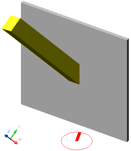
Repeat steps #5 to #8 for all the hours of the Daily Shading Period to create an array of Hourly Shade Solids.
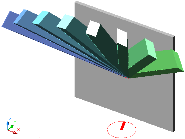
 View this image with your browser for larger size
Phase 4 Define the final shading solid
#10
Merge all Hourly Shade Solids into one using Union. The new solid contains all the solar rays that are directed to the opening during the Daily Shading Period.
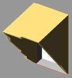
#11
Construct a Device Solid in front of the opening. 
A portion of that solid will become the final shading device.
Make sure that it is large enough to intercept all Hourly Shade Solids of #8
In this example the Device Solid is a yellow rectangular tube perpendicular to the opening, intercepting the blue radial Hourly Shading Solids.
View this image with your browser for larger size
#12
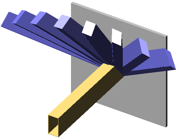
Construct the Intersection of the unified Hourly Shade Solid (#10) and the Device Solid (#11). The new solid prevents all the solar rays from reaching the opening.

Smooth the edges in order to provide shading between hourly steps.

A horizontal overhang with two vertical sides

#13
You can repeat #11 & #12 to test alternative Device Solids.
A horizontal overhang with a vertical slab parallel to the opening A spherical sector with its centre at the bottom of the opening
 
An example The method was developed during a real school design project.
Here is a selection of images produced during the design process:
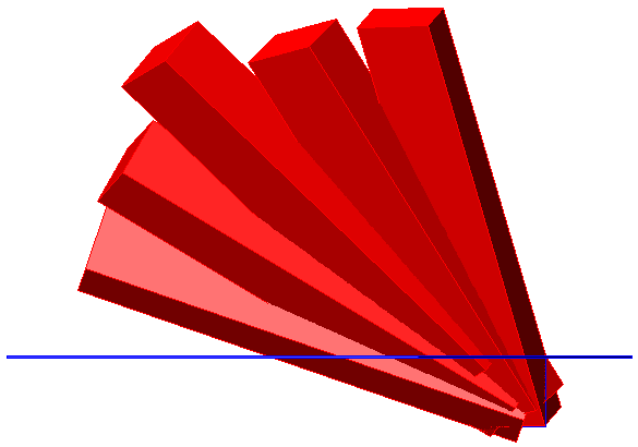
Hourly Shading Solids (red) & horizontal Device Solid (blue) in plan & elevation
 

View this image with your browser for larger sizeView this image with your browser for larger size

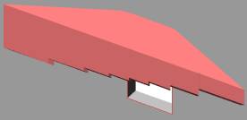
The resulting overhang
View this image with your browser for larger size
Axonometric view of (yellow) overhangs along the SW facing windows of an arcade
(edges have been smoothed)
View this image with your browser for larger size
 
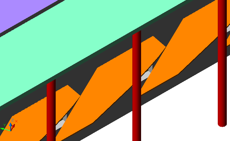
NW elevation with rows of folded perforated metal sheets as shading devices
View this image with your browser for larger size
 
Perspective view of the same NW elevation, with arrays of smaller devices
 
 
Footnote:
The author has developed an AutoLISP algorithm that generates successive 'solar views' of a 3D model according to given input (latitude, orientation, date & solar time steps). Each view can be zoomed-in and stored as AutoCAD View for later reference.
The algorithm has been developed for AutoCAD version 2.62 (1988), so it is independent of Sun Angle Calculator.
For more information please send e-mail.
Solar Envelope -another AutoCAD application by TNS
Contact
TNS main page
This page has been developed by TNS with Netscape composer & MS FrontPage 2000 for a 1024x768 24-bit display.
Posted 13.10.00; last edited 20.09.06